USING A DYNAMIC TIME SERIES MODEL (ARIMA) FOR FORECASTING OF EGYPTIAN COTTON CROP VARIABLES
Mohamed. A. Elsamie1,2, Tarek Ali 3 and Deyi Zhou1*
1College of Economics and Management, Huazhong Agricultural University, Wuhan. 430070, Hubei, P.R. China.
2Department of Agricultural Economics, Faculty of Agriculture, Al-Azhar University, Assuit, P.O. Box 71524 Egypt.
3Agricultural Economics Research Institute, Egypt.
*Corresponding author’s E-mail: zdy@mail.hzau.edu.cn.
ABSTRACT
The Egyptian cotton crop is considered one of the important strategic crops, as it is one of the main pillars of the Egyptian national economic structure, and is used in many local industries, such as the textile industry, oil and soap industry, animal feed etc. Also, the cultivation of this crop employs more than one million workers and earns the Country a lot of foreign exchange from the export of this crop. In the past period, there has been a steady decline in the cultivation; in terms of land area and quantity produced of the crop. To achieve the Aims of this study Used ARIMA models because these models combine the method of Autoregression, the moving average of the time series to the forecasting of the cultivated area, Productivity, and Production of the cotton crop where these models are characterized by high accuracy in the analysis of Time series. We found from the results the cultivated area of that crop reached 230.30 thousand acres in 2018 then decreased to 27.85 thousand acres in 2024. After that the Production of the cotton crop in Egypt will cease because there is no area planted of cotton crop in Egypt after the year 2024. Also, the results of the productivity forecast were 7.06 quintals in 2018 then dropped to 6.61 quintals in 2025. Also, the results of the forecast of Production of the cotton crop reached 1173.61 thousand quintals in 2018 then reduced to 128.33 thousand quintals in 2024. Then after 2024, the Production of Egyptian cotton crop ceased permanently.
Keywords: forecasting, ARIMA model, Moving average model, Cotton crop. Auto-regressive model. Egypt, Auto-correlation function, Partial Auto-correlation Function.
https://doi.org/10.36899/JAPS.2021.3.0271
Published online November 09,2020
INTRODUCTION
The Egyptian cotton crop is considered one of the important strategic crops, as it is one of the main pillars of the Egyptian national economic structure, and participates in many local industries, such as the textile industry, oil and soap industry, animal feed, etc. Also, the cultivation of this crop employs more than one million people. Export of this crop is important to the Egyptian economy because of its comparative advantage and competitiveness in the foreign markets. Besides, the Egyptian cotton crop has an important place in Egyptian history since its emergence in the early 19th century. During Muhammad Ali's rule of the Arab Republic of Egypt, the cultivated of the cotton crop was expanded, and textile factories developed. Where the Egyptian cotton crop competed with the British cotton crop at that time. Foreign exchange earnings of the cotton crop was used in the economic and agriculture development of the country. During the British occupation of Egypt, the important role of the cotton crop declined. Talat Herb, the founder of Bank Masr, re-established the important role of the cotton crop once again affecting Egyptian life.( Abdel Salam,2009), This strategy continued until 1980 when the cultivated varieties of the cotton crop were developed and improved, Productivity increased, and the industrialization of the crop expanded. The Egyptian textile industry during this period achieved significant development at the international level, as well as at the local level. Also, a 20% increase of the cultivated area of the cotton crop was achieved. (Tolpa, 2015)
In 1980 the cultivated area of the cotton crop decreased, as that area reached less than a million acres in 1990. from then, there has been a continuous decline in cultivated area. The decline in the cultivated area continued to reach 1,245 thousand acres in 1980, then 993 thousand acres in 1990, 518 thousand acres in 2000, 369 thousand acres in 2010, then 217 thousand acres in 2017. (MALR, 1980-2017)
Besides, the Egyptian government did not pay attention to improving the varieties of the cotton crop during that period, which led to a decrease in the productivity. This led to a decrease in the comparative advantage and competitive advantage of Egyptian exports of this crop. The continuous decrease in the cultivated area of the cotton crop due to some internal and external factors, as well as technological and economic reasons, such as growing cotton in climatic conditions not suitable for its cultivation, no application of technical recommendations, no pest control, decrease in the production requirements, etc. The main focus of this study includes looking at the developments of the cultivated area, productivity and production of the Egyptian Cotton crop in the future and making proposals and recommendations that will contribute to setting planning and production policies in the future. In this study, the use of different methods for forecasting the economic variables in the future for this crop is ascertained. We used a dynamic time series (ARIMA) model, a combination of the Autoregressive model and moving average model to forecast the cultivated area and productivity and production of the cotton crop in the future. Again, secondary data issued by the Egyptian Government Agencies for both the cultivated area and the productivity and production of the Egyptian cotton crop during the period 1980-2017 were used. (Al-Ani,2005)
The Economic Feasibility of Studying the Egyptian Cotton Crop:
- Egyptian Cotton is of great economic importance as it contributes to agricultural, industrial, internal, and external trade.
- Cotton is considered a cash crop, as it contributes to the national economy.
- The cotton crop needs many agricultural workers; therefore, more than a million workers are into the Production and marketing of the crop.
- The cotton crop provides raw material needed for the textile industry in Egypt.
- The cotton crop consumes very little irrigation water compared to other crops.
- Growing cotton crops on salt intensity lands increases soil fertility.
- The Cotton crop residues is used in the Production of wood and fuel and the cottonseed can be used in oil extraction.
The problem of this study arises because of the marked decrease in the area planted with the cotton crop, especially in recent years. This decrease in productivity and production led to a decrease in the natural characteristics of the Egyptian cotton crop, such as length, softness, and maturity. Also, the quantity of cotton staple imports increased to meet the needs of local consumption. The Egyptian export of cotton crops was also affected by this decline, and the international position of those exports declined. The study aims to predict the cultivated area, productivity and production of the Egyptian cotton crop. ARIMA models were used to contribute to the design of production policies for this crop based on accurate predictive information.
MATERIALS AND METHODS
The study based on the quantitative and descriptive method for the cultivated area, productivity, and production of Egyptian cotton crop during the period (1980-2017) and based on estimating the forecast of the main variables mentioned earlier, through the application of the (ARIMA) model. The (ARIMA) model can provide a short-run estimate for a sufficiently large amount of data on the concerned variables very precisely. The ARIMA model is a combination of three processes:
I. Autoregressive (AR) process.
II. Differencing process
III. Moving-Average (MA) process.
These processes are known in statistical literature as main univariate time series models and are commonly used in many applications. (Abdelrahem,2018)
Autoregressive (AR) Model
An autoregressive model can be expressed as:

Where:
eT: is the error term in the equation
YT: Represent variable values Y Predicted.
YT-1, YT-2, YT-: Represent variable values Y Time-delayed during the T period.
B0 ,B1 ,B2 ,BP : Slope equation coefficients.
The Autoregressive model indicates that the current values of the Y.T. variable depend on the previous variable values YT-1, YT-2, YT-P.
Moving average (MA) model
The Moving average model can be expressed as:

Where
YT: Represent variable values Y predicted.
eT-1, eT-2, eT-q: Represents the lateness of the YT variable estimate.
W0,W1,W2,Wq : Represent weights.
eT: represents the random variable.
From the model, current Y.T. values are based on the previous values of e T-1, e T-2, e T-q
Autoregressive integrated moving average model (ARIMA)
The two previous forms can be grouped into one form called ARIMA.
The new model can be formulated in the following formula:


This form is referred to as ARIMA of the rank (p, q).
Where
P: Refers to the rank of Autoregressive.
q: Refers to the rank of the moving average.
Before applying the above equation to the time series data, we made sure that this series is stable. This means that the dependent variable has an average and constant variation during the study period. If the time series is signed and found to be unstable, it must be converted to a stable series by finding the first difference for this variable as follows:

If the first difference does not result in a stable chain, the first difference to this difference can be taken as follows:

In general, this difference process can be repeated several times until we have a stable chain. So, the ARIMA model is determined by both p d q. ARIMA model (2.1.1) It means it is an Autoregressive model from the Second degree and One difference and one moving average.
Box-Jenkins Models:The time series analysis Approach of the Box - Jenkins Named, after the statisticians George Box and Gwilym Jenkins, applies ARIMA models to find the best fit of a time series model to past values of a time series. (Ahmadzai,2019)
Identification Stage: Ensured that the variables stationary and identifying seasonality in the series, using the Auto-correlation Function and Partial Auto-Correlation Function of the series, to identify Auto-regressive or moving average.
Estimation Stage: Using computation algorithms to arrive at coefficients that best fit the selected ARIMA model.
Diagnostic Stage: By testing whether the estimated model conforms to the specifications of a stationary univariate process the residuals should be independent of each other and constant in mean and variance over time. If the estimation is inadequate, we must return to step one and attempt to build a better model.
Forecasting Stage: Forecasting: When the selected ARIMA model conforms to the specifications of a stationary univariate process, then we can use this model for predicting.
Sources of –Data: The study was based on statistical data published by the Egyptian government agencies issued by the Central Department of Agricultural Economics in the Ministry of Agriculture and Land Reclamation, the Central Authority for Public Mobilization and Statistics and Data of Food and Agriculture Organization ( FAO), some References and related studies to the subject of the study.
RESULTS AND DISCUSSION
Cultivated Area
Identification: The cultivated area for the cotton crop, deduced from the original data, is shown in Figure (1). It is evident that the data series is not static, due to a decreasing of a general trend, which means that the instability of the average by using Auto-correlation function (ACF) and Partial Correlation function (PCF), to detect the stability of the time series. The results indicate in Table (1) the significance of Autocorrelation and partial correlation coefficient values, which indicates that the time series is not static.
Table 1. Autocorrelation and Partial Correlation of cultivated area of the Cotton crop
|
Autocorrelation
|
Partial Correlation
|
|
AC
|
P.A.C.
|
Q-Stat
|
Prob
|
|
. |******|
|
. |******|
|
1
|
0.850
|
0.850
|
29.660
|
0.000
|
|
. |***** |
|
. | . |
|
2
|
0.716
|
-0.021
|
51.308
|
0.000
|
|
. |***** |
|
. |** |
|
3
|
0.668
|
0.231
|
70.658
|
0.000
|
|
. |**** |
|
. | . |
|
4
|
0.612
|
-0.031
|
87.403
|
0.000
|
|
. |**** |
|
. | . |
|
5
|
0.555
|
0.039
|
101.57
|
0.000
|
|
. |**** |
|
.*| . |
|
6
|
0.489
|
-0.068
|
112.94
|
0.000
|
|
. |*** |
|
. | . |
|
7
|
0.441
|
0.041
|
122.50
|
0.000
|
|
. |*** |
|
. | . |
|
8
|
0.392
|
-0.055
|
130.28
|
0.000
|
|
. |** |
|
.*| . |
|
9
|
0.298
|
-0.169
|
134.92
|
0.000
|
|
. |*. |
|
.*| . |
|
10
|
0.184
|
-0.166
|
136.76
|
0.000
|
|
. |*. |
|
. | . |
|
11
|
0.108
|
-0.030
|
137.42
|
0.000
|
|
. | . |
|
. | . |
|
12
|
0.059
|
-0.011
|
137.63
|
0.000
|
|
. | . |
|
. |*. |
|
13
|
0.035
|
0.096
|
137.70
|
0.000
|
|
. | . |
|
. | . |
|
14
|
-0.002
|
-0.030
|
137.70
|
0.000
|
|
. | . |
|
. | . |
|
15
|
-0.035
|
0.041
|
137.78
|
0.000
|
|
. | . |
|
. | . |
|
16
|
-0.045
|
0.044
|
137.92
|
0.000
|
Source: calculated from Table (1) in the Annex.
Fig. 1. Time Series Plot of the cotton area

Source: calculated from Table (1) in the Annex.
Also, by the drawing of the original data of the Auto-correlation function (ACF), we get figure (2). by making the drawing of the original data of the Partial Auto-correlation Function (PACF) for the cultivated area of the cotton crop we get figure (3), The results showed the significance of the Partial Auto-correlation Coefficient, Function., which means rejecting the basic assumption that "the sum of the squares of single correlation coefficients are significant", it means there are correlations Known as full test.

Source: calculated from Table (1) in the Annex.

Source: calculated from Table (1) in the Annex.
Estimation: By examining the Partial Auto-correlation function with the original series as in Figure (3), we find that this parameter falls outside the boundaries of the confidence interval at one gap, Therefore the Auto-regression model (AR) and Moving Average model (MA) must be applied. Finally, the best model is shown in Table (2)
Table 2. Final Estimates of Parameters for cultivated area of the cotton crop (2-1-1).
|
P-value
|
T-value
|
SE Coef
|
Coef
|
Type
|
|
0.050
|
2.03
|
0.1648
|
0.3349
|
AR 1
|
|
0.020
|
-2.44
|
0.1663
|
-0.4056
|
AR 2
|
|
0.000
|
36.68
|
0.0298
|
1.0923
|
MA 1
|
|
0.000
|
-283.16
|
0.09971
|
-28.23415
|
Constant
|
Source: calculated from Table (1) in the Annex.
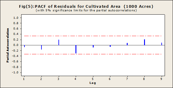
Diagnostic checking:By estimating Auto-correlation function (ACF) and Partial Auto-correlation Function (PACF) of Residuals estimated models (ei), it was found that they are within confidence limits, where it is clear from the two Figures (4) and (5), that there is no specific behavioral pattern for the Auto-correlation function and Partial Auto-correlation function of the Residuals and this indicates the quality of the model.

Source: calculated from Table (1) in the Annex.
Source: calculated from Table (1) in the Annex.
Forecasting: Table (3) shows the results of the forecast of the cultivated area of the cotton crop. The cultivated area reached 230.30 thousand acres in 2018, then decreased to 27.85 thousand acres in 2024, After that the production of the cotton crop in Egypt ceased. The figure shows no area planted of the cotton crop in Egypt after the year 2024.
Table 3. Results of the forecasting for the best dynamic models using Box-Jenkins Models.
|
Year
|
2018
|
2019
|
2020
|
2021
|
2022
|
2023
|
2024
|
2025
|
|
Forecast
(Thousand acres)
|
230.30
|
171.98
|
118.80
|
96.40
|
82.24
|
58.34
|
27.85
|
─
|
Source: calculated from Table (1) in the Annex.
Productivity
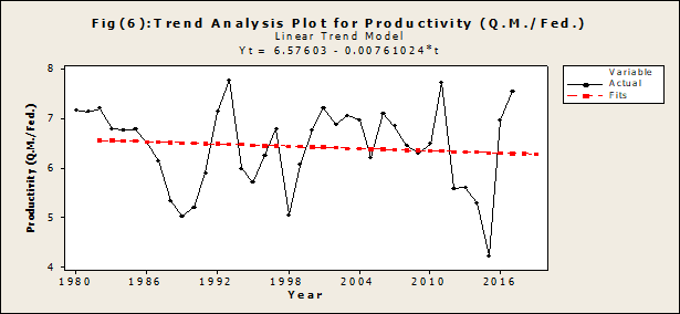
Identification: The Productivity for the cotton crop, deduced from the original data, is shown in Figure (6). It is evident that the data series is not static, due to a decreasing of a general trend, which means that the instability of the average by using Auto-correlation function (ACF) and Partial Correlation function (PCF), to detect the stability of the time series. The results indicate in Table (4) the significance of Autocorrelation and partial correlation coefficient values, which indicates that the time series is not static.
Table 4. Autocorrelation and Partial Correlation of Productivity of the Cotton crop
|
Autocorrelation
|
Partial Correlation
|
|
AC
|
P.A.C.
|
Q-Stat
|
Prob
|
|
****| . |
|
****| . |
|
1
|
-0.495
|
-0.495
|
9.5785
|
0.002
|
|
.*| . |
|
***| . |
|
2
|
-0.079
|
-0.430
|
9.8316
|
0.007
|
|
. |*. |
|
**| . |
|
3
|
0.131
|
-0.225
|
10.539
|
0.014
|
|
.*| . |
|
**| . |
|
4
|
-0.120
|
-0.295
|
11.153
|
0.025
|
|
. |*. |
|
.*| . |
|
5
|
0.135
|
-0.098
|
11.958
|
0.035
|
|
.*| . |
|
**| . |
|
6
|
-0.184
|
-0.317
|
13.494
|
0.036
|
|
. |*. |
|
.*| . |
|
7
|
0.198
|
-0.077
|
15.339
|
0.032
|
|
.*| . |
|
.*| . |
|
8
|
-0.074
|
-0.108
|
15.606
|
0.048
|
|
.*| . |
|
**| . |
|
9
|
-0.138
|
-0.264
|
16.568
|
0.056
|
|
. |** |
|
.*| . |
|
10
|
0.230
|
-0.120
|
19.346
|
0.036
|
|
. | . |
|
. | . |
|
11
|
-0.044
|
0.069
|
19.453
|
0.053
|
|
. | . |
|
. |*. |
|
12
|
-0.049
|
0.114
|
19.589
|
0.075
|
|
.*| . |
|
.*| . |
|
13
|
-0.136
|
-0.143
|
20.685
|
0.079
|
|
. |*. |
|
. | . |
|
14
|
0.181
|
-0.021
|
22.716
|
0.065
|
|
. | . |
|
. | . |
|
15
|
-0.032
|
-0.050
|
22.783
|
0.089
|
|
.*| . |
|
. | . |
|
16
|
-0.087
|
-0.058
|
23.299
|
0.106
|
Source: calculated from Table (1) in the Annex
Fig. 6. Time Series Plot of Productivity of the Cotton crop.
Source: calculated from Table (1) in the Annex
Also, by the drawing of the original data of the Auto-correlation function (ACF), we get figure (7). Making the drawing of the original data of the Partial Auto-correlation Function (PACF) for Productivity of the cotton crop we get figure (8), The results showed the significance of the Partial Auto-correlation Coefficient, Function., which means rejecting the basic assumption that "the sum of the squares of single correlation coefficients are significant", it means there are correlations known as full test.

Source: calculated from Table (1) in the Annex

Source: calculated from Table (1) in the Annex
Estimation: By examining the Partial Auto-correlation function with the original series as in Figure (8), we find that this parameter falls outside the boundaries of the confidence interval at one gap. Therefore, the Auto-regression model (AR) and Moving Average model (MA) must be applied. Finally, the best model is shown in Table (5).
Table 5. Final Estimates of Parameters for Productivity of the Cotton crop (1-1-1)
|
P-value
|
T-value
|
SE Coef
|
Coef
|
Type
|
|
0.004
|
3.05
|
0.1609
|
0.4901
|
AR 1
|
|
0.000
|
13.14
|
0.0793
|
1.0419
|
MA 1
|
|
0.785
|
0.28
|
0.008973
|
0.002471
|
Constant
|
Source: calculated from Table (1) in the Annex.
Diagnostic checking: By estimating Auto-correlation function (ACF) and Partial Auto-correlation Function (PACF) of Residuals estimated models (ei), it was found that they are within confidence limits, where it is clear from the two Figures (9) and (10), that there is no specific behavioral pattern for the Auto-correlation function and Partial Auto-correlation function of the Residuals and this indicates the quality of the model.

Source: calculated from Table (1) in the Annex.

Source: calculated from Table (1) in the Annex
Forecasting:Table (6) shows the results of productivity forecast were 7.06 quintals in 2018 then dropped to 6.61 quintals in 2025.
Table 6. Results of the forecasting for the best dynamic models using Box-Jenkins Models.
|
Year
|
2018
|
2019
|
2020
|
2021
|
2022
|
2023
|
2024
|
2025
|
|
Forecast
(Quintals)
|
7.0569
|
6.8128
|
6.6957
|
6.6407
|
6.6163
|
6.6067
|
6.6045
|
6.6059
|
Source: calculated from Table (1) in the Annex.
The Production
Identification: The Production for the cotton crop, deduced from the original data, is shown in Figure (11). It is evident that the data series is not static, due to a decreasing of a general trend, which means that the instability of the average by using Auto-correlation function (ACF) and Partial Correlation function (PCF), to detect the stability of the time series. The results indicate in Table (7) the significance of Autocorrelation and partial correlation coefficient values, which indicates that the time series is not static.
Table 7. Autocorrelation and Partial Correlation of Production of the Cotton crop
|
Autocorrelation
|
Partial Correlation
|
|
AC
|
P.A.C.
|
Q-Stat
|
Prob
|
|
. |******|
|
. |******|
|
1
|
0.791
|
0.791
|
25.720
|
0.000
|
|
. |**** |
|
. | . |
|
2
|
0.617
|
-0.025
|
41.773
|
0.000
|
|
. |**** |
|
. |*. |
|
3
|
0.558
|
0.209
|
55.310
|
0.000
|
|
. |**** |
|
. | . |
|
4
|
0.521
|
0.057
|
67.462
|
0.000
|
|
. |*** |
|
. | . |
|
5
|
0.460
|
-0.006
|
77.203
|
0.000
|
|
. |** |
|
.*| . |
|
6
|
0.349
|
-0.138
|
82.995
|
0.000
|
|
. |** |
|
. | . |
|
7
|
0.294
|
0.062
|
87.238
|
0.000
|
|
. |** |
|
.*| . |
|
8
|
0.244
|
-0.077
|
90.245
|
0.000
|
|
. |*. |
|
. | . |
|
9
|
0.203
|
0.032
|
92.399
|
0.000
|
|
. |*. |
|
.*| . |
|
10
|
0.146
|
-0.068
|
93.551
|
0.000
|
|
. |*. |
|
. | . |
|
11
|
0.110
|
0.047
|
94.236
|
0.000
|
|
. |*. |
|
. | . |
|
12
|
0.077
|
-0.064
|
94.580
|
0.000
|
|
. | . |
|
. | . |
|
13
|
0.020
|
-0.053
|
94.606
|
0.000
|
|
. | . |
|
. | . |
|
14
|
-0.011
|
-0.005
|
94.614
|
0.000
|
|
. | . |
|
. | . |
|
15
|
-0.029
|
0.005
|
94.670
|
0.000
|
|
. | . |
|
. | . |
|
16
|
-0.022
|
0.044
|
94.703
|
0.000
|
Source: calculated from Table (1) in the Annex
Fig. 11. Time Series Plot of Production of the cotton crop

Source: calculated from Table (1) in the Annex
Also, by the drawing of the original data of the Auto-correlation function (ACF), we get figure (12). Making the drawing of the original data of the Partial Auto-correlation Function (PACF) for Production of the cotton crop we get figure (13), The results showed the significance of the Partial Auto-correlation Coefficient, Function., which means rejecting the basic assumption that "the sum of the squares of single correlation coefficients are significant", it means there are correlations known as full test.

Source: calculated from Table (1) in the Annex

Source: calculated from Table (1) in the Annex
Estimation: By examining the Partial Auto-correlation function with the original series as in Figure (13), we find that this parameter falls outside the boundaries of the confidence interval at one gap. Therefore, the Auto-regression model (AR) and Moving Average model (MA) must be applied. Finally, the best model is shown in Table (8).
Table 8. Final Estimates of Parameters for Production of the Cotton crop (0-1-1).
|
P-value
|
T-value
|
SE Coef
|
Coef
|
Type
|
|
0.000
|
11.19
|
0.0854
|
0.9562
|
MA 1
|
|
0.000
|
-13.45
|
12.95
|
-174.21
|
Constant
|
Source: calculated from Table (1) in the Annex.
Diagnostic Checking: By estimating Auto-correlation function (ACF) and Partial Auto-correlation Function (PACF) of Residuals estimated models (ei), it was found that they are within confidence limits, where it is clear from the two Figures (14) and (15) that there is no specific behavioral pattern for the Auto-correlation function and Partial Auto-correlation function of the Residuals and this indicates the quality of the model.

Source: calculated from Table (1) in the Annex.

Source: calculated from Table (1) in the Annex.
Forecasting: Table (9) shows the results of the forecast of Production of the cotton crop which reached 1173.61 thousand quintals in 2018, then reduced to 128.33 thousand quintals in 2024. Then after 2024, the Production of the cotton crop of Egypt ceased permanently.
Table 9. Results of the forecasting for the best dynamic models using Box-Jenkins Models.
|
Year
|
2018
|
2019
|
2020
|
2021
|
2022
|
2023
|
2024
|
2025
|
|
Forecast
(thousand quintals)
|
1173.61
|
999.39
|
825.18
|
650.97
|
476.76
|
302.55
|
128.33
|
-45.88
|
Source: calculated from Table (1) in the Annex.
Conclusion and Recommendations: The Egyptian cotton crop is considered one of the important strategic crops, as it is one of the main pillars of the Egyptian national economic structure, Also, the cultivation of this crop employs more than one million workers, To achieve the Aims of this study, we used ARIMA models because these models combine the method of Autoregression, the moving average of the time series to the forecasting of the cultivated area, productivity, and production of the cotton crop where these models are characterized by high accuracy in the analysis of Time series, We found from the results the cultivated area of that crop reached 230.30 thousand acres in 2018, then decreased to 27.85 thousand acres in 2024. After that, the production of the cotton crop in Egypt will cease because there will be no area planted of cotton crop in Egypt after the year 2024. Also, the results of the productivity forecast were 7.06 quintals in 2018, and then dropped to 6.61 quintals in 2025. Also, the results of the forecast of production of the cotton crop the production reached 1173.61 thousand quintals in 2018, then reduced to 128.33 thousand quintals in 2024. Then after 2024, the production of Egyptian cotton crop will cease permanently.
Based on the research results, we recommend the following:
i. Reducing production costs by assessing the real costs of production inputs, eliminating or rationalizing administrative costs.
ii. Study support methods in cotton crop-producing countries, such as India, Pakistan, the United States, and Brazil, and their application in Egypt.
iii. Improving productivity through many factors, such as the production of new varieties that promote acres productivity.
iv. Importing new genetic assets to hybridize with Egyptian Cotton.
v. The government sets a forced price for the cotton crop.
vi. Providing the cotton crop production requirements, such as fertilizers and pesticides at affordable prices.
vii. Activating the role of agricultural guides in educating producers about harvesting and packing, and not using sisal filaments in sewing cotton bags.
viii. Identify a tripartite agricultural cycle to eliminate randomness in agriculture.
ix. Encourage the use of agricultural mechanization in cotton crop cultivation, from agriculture to harvesting.
ANNEX
Table 1. Economic variables of the Egyptian cotton crop over the period 1980-2017.
|
Production
(Thousand quintals)
|
Productivity
(Quintals)
|
Area
(Thousand acres)
|
Years
|
|
8941.38
|
7.18
|
1244.53
|
1980
|
|
8413.92
|
7.14
|
1178.42
|
1981
|
|
7684.71
|
7.21
|
1065.84
|
1982
|
|
6788.30
|
6.80
|
998.28
|
1983
|
|
6658.70
|
6.77
|
983.56
|
1984
|
|
7340.06
|
6.79
|
1081.01
|
1985
|
|
6898.78
|
6.54
|
1054.86
|
1986
|
|
6025.71
|
6.15
|
979.79
|
1987
|
|
5424.69
|
5.35
|
1013.96
|
1988
|
|
5057.82
|
5.03
|
1005.53
|
1989
|
|
5173.79
|
5.21
|
993.05
|
1990
|
|
5022.55
|
5.90
|
851.28
|
1991
|
|
6008.07
|
7.15
|
840.29
|
1992
|
|
6879.93
|
7.78
|
884.31
|
1993
|
|
4328.64
|
6.00
|
721.44
|
1994
|
|
4062.40
|
5.72
|
710.21
|
1995
|
|
5764.90
|
6.26
|
920.91
|
1996
|
|
5842.97
|
6.80
|
859.26
|
1997
|
|
3983.84
|
5.05
|
788.88
|
1998
|
|
3917.70
|
6.07
|
645.42
|
1999
|
|
3514.10
|
6.78
|
518.32
|
2000
|
|
5285.90
|
7.23
|
731.11
|
2001
|
|
5565.90
|
6.88
|
706.41
|
2002
|
|
3783.10
|
7.07
|
535.09
|
2003
|
|
4981.70
|
6.97
|
714.73
|
2004
|
|
4084.00
|
6.22
|
656.59
|
2005
|
|
3808.40
|
7.10
|
536.40
|
2006
|
|
3941.60
|
6.86
|
574.57
|
2007
|
|
2020.10
|
6.46
|
312.71
|
2008
|
|
1791.90
|
6.30
|
284.43
|
2009
|
|
2395.70
|
6.49
|
369.14
|
2010
|
|
4025.70
|
7.74
|
520.12
|
2011
|
|
1863.50
|
5.59
|
333.36
|
2012
|
|
1608.50
|
5.61
|
286.72
|
2013
|
|
1956.70
|
5.30
|
369.18
|
2014
|
|
1016.50
|
4.22
|
240.87
|
2015
|
|
918.30
|
6.97
|
131.75
|
2016
|
|
1640.10
|
7.56
|
216.95
|
2017
|
Source: Calculated using on data collected from the Ministry of Agriculture and Land Reclamation, Economic
Affairs Sector, Central Administration for Agricultural Economics, Bulletin of Agricultural Economics;
Different Issues.
Table 2. The average and standard deviation of cultivated area, Productivity, and Production of the Egyptian cotton crop.
|
Variables
|
N
|
Minimum
|
Maximum
|
Mean
|
Std. Deviation
|
CV
|
|
Area
(Thousand acres)
|
38
|
131.75
|
1244.53
|
706.82
|
301.72
|
42.69
|
|
Productivity
(Quintals)
|
38
|
4.22
|
7.78
|
6.43
|
0.83
|
12.91
|
|
production
(Thousand quintals)
|
38
|
918.30
|
8941.38
|
4590.01
|
2095.55
|
45.65
|
Source: calculated from Table (1) in the Annex.
REFERENCES
- Abdel Salam, Mohamed, E. (2009). Promotion of Cotton in the national economy. Egyptian Cotton Crisis Symposium. Egypt. J. Agri. Sci.
- Abdelmola, Khaled, E, (2018). An economic study of organic cotton crop in Egypt, Egypt. J. Agri Sci, 28(2):647-662.
- Abdelrahem Hesham A, (2018). An economic study of the impact of some agricultural Policies on Cotton and rice crops, Egypt. J. Agri. Sci,28(2):663-686.
- Abdul Maksoud, Abdullah, M, (2003). Demand for Egyptian Cotton in international markets.Ph.d.Sc. Thesis (unpublished). Deptt. Of Agri. Economics, Univ. Agri., Ain-Shams.
- Ahmadzai, M. Karim (2019). Using ARIMA Models to Forecasting of Economic Variables of Wheat Crop in Afghanistan, AJEBA, 13(4): 1-21.
- Ahmed, Yousry, N, (2015). Estimating indicators of Egyptian cotton production during the period 1980-2013 future political scenarios, M.Sc. Thesis unpublished). Deptt of Agri. Economics., Univ. Agri., Cairo.
- Al Shuwaikh, Dalia, H (2015). An economic study of the determinants of supply Response to cotton yield in Egypt. Assiut. J. Agri. Sci. 46(6): 104-120.
- Al-Ani, Ahmed, H (2005). The use of ARIMA models in economic forecasting. Department of Economics. College of Administration and Economics. Univ, Anbar.
- Aldali, Kamal, S. (2014). The role of agricultural policy in the Production of Egyptian Cotton. Mansoura. J.Agri. Sci. 5(1): 89-101.
- Al-Gendi, Mohamed, S. (2016). An economic study for the Production and marketing of Cotton in the Arab Republic of Egypt. Mansoura. J. Agri. Sci. 7(5): 539-544.
- Al-Zenati, Al- Metwali, S. (2014). Analytical Study of Factors Affecting Cotton Production in Egypt. Egypt. J. Agri. Sci, 24 (2).
- Attia, Rehan, M (2018). An Economic Study of Problems Facing Cotton Production in Egypt (Case Study of Abu Homs, Beheira Governorate). Mansoura. J. Agri. Sci. 9(2): 117-123.
- CAPMAS, (1980-2017). Foreign Trade Database, Foreign Trade Bulletins, Govt. Egypt. Cairo.
- Darwish, Mohyee, Z, (2018). an analytical economic study of the factors affecting the future of Egyptian cotton production, Egypt. J. Agri. Sci, 28(9):1233-1250.
- El Sayed, Hebat Allah, A, (2016). The economics of Egyptian Cotton under the current situation. Mansoura. J. Agri. Sci. 7(9): 899-905.
- Elhosany, Lamyaa, S. (2014). Problems facing cotton farmers in some villages of Kafr El-Sheikh governorate. Mansoura. J. Agri. Sci. 5(6): 993-1013.
- Elsamie, A. Mohamed (2020). Impact of Agricultural Policies on the Egyptian Cotton Sector using Policy Analysis Matrix, Asian J. Econ. Business Accounting, 15(1): 50-59.
- Emara, Riyad, (2015). Egyptian cotton present and future, Mansoura. J. Agri. Sci. 6(10):1611-1624.
- Food and Agriculture Organization (FAO).
- Ibrahim, Wajdi, H (2009). International Trade of Cotton. Egyptian Cotton Crisis Symposium. Egypt. J. Agri. Sci.
- Ibrahim, Wajdi, H (2015). The future of Egyptian Cotton and its economics of Production, manufacturing, and trade internally and externally. Symposium on The Future of Egyptian Cotton.
- Kamra, Sahar, A. (2014). Estimation of the current and projected economic price of the Cotton crop in Egypt. Mansoura. J. Agri. Sci. 5(4): 501-515.
- MALR, (1980-2017). Economic Affairs Sector, the Central Administration for Agricultural Economics, Bulletin of Agricultural Economics, Govt. Egypt., Giza.
- Mansour, Fatma, A, (2017). The standard analysis of cotton area limits in Egypt, Mansoura. J. Agri. Sci, 8(10):659-664.
- Nassar, Saad (2015). Egyptian Cotton or white gold to where? Egypt. J. Agri. Sci.
- Nejm, Mohamed, A. (2015). Urgent measures to promote Egyptian Cotton as the main Crop. Symposium on the Future of Egyptian Cotton. Statistical database on the WTO. Website.
- Tolpa, Ahmed, A, (2015). Cotton Marketing Policy in Egypt: Problems and Solutions. A working paper submitted to the Agricultural Economics Research Institute, MALR, Egypt.
- Youssef. Hind, N. (2001). An economic study to liberalize cotton production and Marketing in Egypt.M.Sc. Thesis (unpublished). Deptt. Of Agri. Economics., Univ. Agri., Zagazig.
|