SPAWNING SEASON, SEASONAL CONDITION FACTOR AND ALLOMETRIC GROWTH PATTERN OF CHAENOGOBIUS GULOSUS (SAUVAGE, 1882) INHABITING ROCKY SUBTIDAL HABITATS IN THE SOUTH-EASTERN KOREA
J. M. Park1 and J. M. Jeong2*
1 Dokdo Research Center, East Sea Research Institute, Korea Institute of Ocean Science & Technology, Uljin 36315, Korea
2 Fisheries Resources Research Center, National Institute of Fisheries Science, Tongyeong 56034, Korea
*Corresponding author’s email: jaemookjeong@korea.kr
ABSTRACT
This study presents data on spawning season, length-weight and length-length relationships, and seasonal condition factors of Chaenogobius gulosus (Sauvage, 1882) inhabiting rocky subtidal habitat in the south-eastern Korea. Monthly changes in the gonadosomatic index (GSI) indicated that the spawning period was from December to April. Values of the exponent b, estimated by nonlinear least squares from weight and length data, ranged from 2.860 for mature group to 3.184 for immature fishes, but it was similar between spawning and non-spawning seasons, and between female and male fishes. All relationships between total and standard length were linear (r2> 0.947). The condition factors were significantly higher during the spawning season than during the non-spawning season, but those were not significant between immature and mature groups, and between female and male fishes. The results from this study can contribute to increasing our knowledge on biology of C. gulosus, and are useful data for conservation and management of this species.
Keywords: Chaenogobius gulosus, condition factor, LLR, LWR, Tongyeong.
https://doi.org/10.36899/JAPS.2020.5.0147
Published online June 25, 2020
INTRODUCTION
Measuring body morphometrics of fishes is a basic procedure in fishery sciences, because fishery species can identify and compare specific species, populations and stocks via morphometric relationships (King, 1995; Froese, 1998). The exponential parameter (b) and intercept (a) of length-weight relationship (LWR) and length-length relationship (LLR) parameters (a, b) have been applied in assessing fish stocks and populations (Ricker, 1968). For example, LWRs are useful to predict the average weight at a given length group and convert length data into weights to provide a measure of biomass (or vice versa) (Froese, 2006; Froese et al., 2011), because stock assessment models and management for fisheries require information about body weight for estimation and regulation of catches (Froese et al., 2014). LLRs are also important for comparative growth studies among taxonomical similar species (Moutopoulos and Stergiou, 2002). Fulton’s condition factor is widely used to measure the health, i.e. fish well-being, and seasonal body condition of individual fish (Le Cren, 1951; Froese, 2006). This factor is based on the hypothesis that for a given length, heavier fishes are in better condition than lighter fishes, and fatness is used as a measure of fish health (Bagenal and Tesch, 1978).
Chaenogobius gulosus is a member of the family Gobiidae and mainly distributed in the shallow coastal area of western Pacific including Korea peninsula, Japan and Yellow Sea (Yamada et al., 1986; Kim et al., 2005).The species usually lives between rock matrices in subtidal zone of the temperate coastal area (Kim et al., 2005), and mainly consumed various rock-dwelling macro-invertebrates as well as seaweeds (Baeck et al., 2010). Although C. gulosus is not commercially caught, they are potential food resources for larger coastal residents such as rosefish Helicolenus hilgendorfii and scorpion fish Sebastiscus marmoratus (Baeck et al., 2011b, 2013). Several studies on biometric relationships and seasonal condition factors for gobies have been conducted globally (e.g. Hossain et al., 2009; Ghanbarifardi et al., 2015; Dinh, 2016), but a little is known regarding LWR and LLR parameters for Korean gobiid fishes. Only a few studies are available on the biometric relationships of this group of fishes in Korea (e.g. Baeck and Park, 2015; Park and Huh, 2015). In this paper, we provide the first LWR and LLR values and seasonal condition factors, and new maximum length for C. gulosus.
MATERIALS AND METHODS
Samplings: Fish specimens were collected in the rocky subtidal habitat of the south-eastern Korea (34°50′N, 127°33′E; Fig. 1). Samplings were conducted monthly from October 2008 to September 2009 during high tide of spring tide in each month and fish samples were collected using a shore-angling by dropping fishing hook between rocky matrices and then striking fishes. The tidal range during spring tide is approximately 1.8 m in the study area. Immediately after capture, individuals were snap frozen and taken to the laboratory. Total length (TL), standard length (SL), and wet body weight (BW) were measured to the nearest millimeter and nearest gram, respectively. The peritoneum of each fish specimen was excised, and the gonads were removed and weighed to the nearest 0.0001 g (GW). Sex was determined macroscopically by examining gonads. Fish maturity was estimated according to maturity size (i.e. immature, <8.0 cm SL; mature ≥8.0 cm SL), following Baeck et al. (2011a).
Data analysis: The gonadosomatic index (GSI) was calculated as follows: GSI = (GW/BW) × 100, where GW is gonad weight (g) and BW is body weight (g). One-way analysis of variance (ANOVA) followed by Tukey’s post-hoc comparisons were used to assess whether there were significant differences of GSIs among months.
For each species, the length-weight function, BW = aTLb, was fitted to the data using linear regressions of log10-transformed data, where BW represents wet body weight (g), TL is total length (cm), and a and b are the intercept and allometric coefficient, respectively. Extreme outliers were removed before fitting the regression because the data were increased measurement errors (Froese et al., 2011). The relationships between TL and SL were established using the linear regression function TL = a + bSL. The standard error (SE) of parameters a and b, and the statistical significance level of r2 were estimated. We summarized LWR and LLR values in each seasons (spawning and non-spawning), maturities (immature and mature; Baeck et al., 2011a), genders (female and male), and all specimens combined. Analyses of covariance (ANCOVA) was used to test the effect of the categorical factors of season, maturity and gender in the relationships between body weight and total length. The relationships between BW and TL, and between TL and SL, and interactions between categorical factors and covariates on these relationships were investigated by ANCOVA.
The Fulton’s condition factor (K) was calculated for each fish according to the equation K = 100 × BW/SL3 (Pauly, 1984; Froese, 2006). Differences in condition factors were examined with respect to season, maturity and gender. The assumptions of normality and homoscedasticity were met for the species (P > 0.05); three-way analysis of variances (ANOVAs) was used to assess whether there were significant influences on condition factor by season, maturity and gender as well as their two-way and three-way interactions. All statistical analyses were performed using SYSTAT software (Systat version 12.0, SPSS Inc., Chicago, IL, USA). An assumed significance level of 0.05 was used in all statistical analyses.
RESULTS
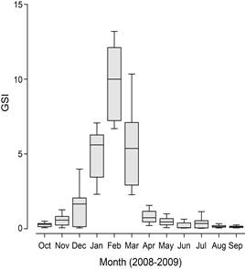
Monthly GSI values of female began to increase in December, reaching the highest level in February and decreasing thereafter (Fig. 2). ANOVA results showed that GSI values were significantly different among months, with the highest value in February, followed by January and March (ANOVA post-hoc test, P < 0.05). On the other hand, those of male did not change significantly among months (ANOVA, P > 0.05). Gonad development of female C. gulosus began in December, with spawning taking place primarily between December and April.
Length-weight and length-length regressions were applied to 330 specimens of C. gulosus. The estimated parameters of LWR and LLR, and descriptive statistics by season, maturity and gender and all fishes, are provided in Table 1. All LWRs were highly significant (P < 0.05), with r2 values >0.872. The r2 values ranged from 0.872 for mature group to 0.990 for individuals during the non-spawning period. ANCOVA results revealed that the slope (b-value) of the LWR did not differ significantly between non-spawning and spawning season, and between genders, but it was significant between immature and mature groups, with higher value for immature fishes than mature group (P < 0.05). The LLR values were highly correlated for all relations among the two length measurements (r2 > 0.947, P < 0.05).
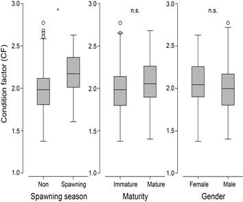
The mean seasonal values of condition factors of C. gulosus were 1.983 during non-spawning season and 2.161 during spawning, and showed significantly higher value the latter period (P < 0.05), but there were no significant two- and three-way interactions among categorical factors of season, maturity and gender (three-way ANOVAs, P > 0.05; Fig. 3).
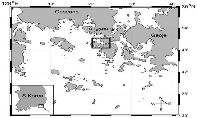
Fig. 1. Location of sampling area in the south-eastern Korean waters. Samples were collected along the shore lines within boxed area.
 |
 |
|
Fig. 2. Monthly changes in GSI of female Chaenogobius gulosus inhabiting rocky subtidal habitats in the south-eastern Korea.
|
Fig. 3. Box plots of condition factors for Chaenogobius gulosus in relation to spawning, maturity and gender. Open cycles represent outliers. *=statistical significance at 0.05, n.s.=no significance.
|
Table 1. Length-weight relationship (LWR) and length-length relationship (LLR) parameters of Chaenogobius gulosus inhabiting rocky subtidal habitat in the south-eastern Korea.
|
Factors
|
N
|
SL (cm)
|
TL (cm)
|
BW (g)
|
W=aLb
|
TL = a + bSL
|
|
A
|
SE
|
b
|
SE
|
r2
|
ANCOVA
|
a
|
SE
|
b
|
SE
|
r2
|
ANCOVA
|
|
Season
|
|
Non-spawning
|
248
|
2.0-11.8
|
2.4-14.0
|
0.11-37.55
|
0.0088
|
0.019
|
3.135
|
0.020
|
0.990
|
0.142
|
0.243
|
0.043
|
1.150
|
0.005
|
0.995
|
0.162
|
|
Spawning
|
82
|
6.4-12.6
|
7.8-14.7
|
5.91-45.35
|
0.0100
|
0.110
|
3.103
|
0.101
|
0.916
|
0.667
|
0.252
|
1.117
|
0.027
|
0.957
|
|
Maturity
|
|
Immature
|
122
|
2.0-7.9
|
2.4-9.6
|
0.11-11.88
|
0.0081
|
0.029
|
3.184
|
0.036
|
0.985
|
<0.001
|
0.165
|
0.062
|
1.166
|
0.011
|
0.989
|
0.035
|
|
Mature
|
208
|
8.0-12.6
|
9.4-14.7
|
10.30-45.35
|
0.0175
|
0.080
|
2.860
|
0.086
|
0.872
|
0.578
|
0.177
|
1.119
|
0.018
|
0.947
|
|
Gender
|
|
Female
|
152
|
2.0-12.6
|
2.4-14.7
|
0.11-45.35
|
0.0086
|
0.026
|
3.157
|
0.027
|
0.989
|
0.914
|
0.182
|
0.065
|
1.166
|
0.008
|
0.993
|
0.069
|
|
Male
|
178
|
2.4-12.1
|
3.0-14.2
|
0.31-38.43
|
0.0085
|
0.026
|
3.151
|
0.027
|
0.987
|
0.273
|
0.063
|
1.146
|
0.007
|
0.993
|
|
Total
|
330
|
2.0-12.6
|
2.4-14.7
|
0.11-47.35
|
0.0086
|
0.017
|
3.155
|
0.018
|
0.990
|
0.023
|
0.046
|
1.155
|
0.005
|
0.993
|
N=number of individuals, SL=standard length, TL=total length, BW=wet body weight, a=intercept, b=slope, r2=coefficient of determination, SE=standard error.
DISCUSSION
The length-weight and length-length regressions for many fish species are available in FishBase, a global biological database on fishes (Froese and Pauly, 2017). Our result provides the first quantitative LWR and LLR estimates for C. gulosus, and also gives new maximum length for C. gulosus (i.e. 12.6 cm SL and 14.7 cm TL). The estimated b values from this study were within the standard range of 2.5-3.5 which indicate for the majority of fish species (Froese, 2006). The b values were the higher end of the expected range, indicating towards positive allometry, but that of mature group was shown negative allometry.
In this study, the condition factors were significantly different between non-spawning and spawning, but not between maturities or genders. Because there were no significant interactions among those factors, variations of condition factor of this species were attributed to seasonal changes in body condition in relation to spawning behavior and/or food intakes. Seasonal changes in body condition were related with seasonal variations in energy reserves (protein, lipid, glycogen and total energy) which are usually driven by food availability, environmental conditions, and reproductive status (Chellappa et al., 1995; Weatherley and Gill, 1987). Fulton’s condition factor differed seasonally in many fish species because of fluctuations in food availability and environmental conditions, consequently, changes in food reserves throughout the year (Hossain, 2010; Lavergne et al., 2013). While several goby species such as Periophthalmus barbarus and Trypauchen vagina showed relatively low condition factor during the breeding season (e.g. King and Udo, 1998; Chukwu and Deekae, 2011; Dinh, 2016). In some goby species (e.g. Periophthalmus mudskippers), low condition factors in breeding season were results from insufficient available food resources and limited foraging opportunities for guarding parents that remain in the space adjacent to the burrow (Colombini et al., 1996; Baeck and Park, 2015). Thus, seasonal changes of body condition look species-specific at least gobiid fishes.
Conclusion: This study provides data on the spawning season, LWR, LLR, and seasonal condition factors of C. gulosus captured from rocky subtidal habitat in the south-eastern Korea. These results contribute towards future conservation studies of the species, and be useful for fishery biologists and managers in Korea.
Acknowledgments: We would like to thank to Mr. Sang Jin Ye for his assistancein the sample collection and measurement of fish samples. This research was supported by a grant from the National Institute of Fisheries Science, Korea (R2020021).
REFERENCES
- Baeck, G.W., and J.M. Park (2015). Length-weight and length-length relationships and seasonal condition factors for two mudskippers, Periophthalmus modestus (Cantor, 1842) and P. magnuspinnatus (Lee, Choi & Ryu, 1995) (Gobiidae), on tidal flats of Korea. J. Appl. Ichthyol. 31(1): 261–264.
- Baeck, G.W., C.I. Park, J.M. Jeong, M.C. Kim, S.H. Huh, and J.M. Park (2010). Feeding habits of Chaenogobius gulosus in the coastal waters of Tongyeong, Korea. Korean J. Ichthyol. 22(1): 41–48.
- Baeck, G.W., J.M. Jeong, J.M. Park, and S.H. Huh (2011a). Reproductive characteristic of gluttonous goby, Chaenogobius gulosus in the coastal waters of Tongyeong, Korea. Korean J. Ichthyol. 23(4): 300–304.
- Baeck, G.W., J.M. Park, H.C. Choi, and S.H. Huh (2013). Diet composition in summer of rosefish Helicolenus hilgendorfii on the southeastern coast of Korea. Ichthyol. Res. 60(1), 75–79.
- Baeck, G.W., Y.M. Yeo, J.M. Jeong, J.M. Park, and S.H. Huh (2011b). Feeding habits of scorpion fish, Sebastiscus marmoratus, in the coastal waters of Tongyeong, Korea. Korean J. Ichthyol. 23(2): 128–134.
- Bagenal, T.B., and A.T. Tesch (1978). Conditions and Growth Patterns in Freshwater Habitats. Blackwell Scientific Publication, Oxford, pp. 75–89.
- Chellappa, S., F.A. Huntingford, R.H.C. Strang, and R.Y. Thomson (1995). Condition factor and hepatosomatic index as estimates of energy status in male three‐spined stickleback. J. Fish Biol. 47(5): 775–787.
- Chukwu, K., and S. Deekae (2011). Length-weight relationship, condition factor and size composition of Periophthalmus barbarus (Linneaus 1766) in New Calabar River, Nigeria. Agric. Biol. J. N. Am. 2(7): 1069–1071.
- Colombini, I., R. Berti, A. Nocita, and L. Chelazzi (1996). Foraging strategy of the mudskipper Periophthalmus sobrinus Eggert in a Kenyan mangrove. J. Exp. Mar. Biol. Ecol. 197(2): 219–235.
- Dinh, Q.M. (2016). Growth pattern and body condition of Trypauchen vagina in the Mekong Delta, Vietnam. J. Anim. Plant Sci. 26(2): 523–531.
- Froese, R. (1998). Length-weight relationships for 18 less-studied fish species. J. Appl. Ichthyol. 14(1–2): 117–118.
- Froese, R. (2006). Cube law, condition factor and weight-length relationships: history, meta–analysisand recommendations. J. Appl. Ichthyol. 22(4): 241–253.
- Froese, R., and D. Pauly (Eds) (2017). FishBase. World Wide Web electronic publication. version (10/2017). Available at: http://www.fishbase.org.
- Froese, R., A.C. Tsikliras, and K.I. Stergiou (2011). Editorial note on Weight–Length relations of fishes. Acta Ichthyol. Piscat. 41(4): 261–263.
- Froese, R., J.T. Thorson, R.G. jr. Reyes (2014). A Bayesian approach for estimating length–weight relationships in fishes. J. Appl. Ichthyol. 30(1): 78–85.
- Ghanbarifardi, M., S. Ghasemian, M. Aliabadian, and A. Pehpuri (2015). Length–weight relationships for three species of mudskippers (Gobiiformes: Gobionellidae) in the coastal areas of the Persian Gulf and Gulf of Oman, Iran. Iran. J. Ichthyol. 1(1): 29–31.
- Hossain, M.Y. (2010). Length-weight, length-length relationships and condition factor of three Schibid catfishes from the Padma River, Northwestern Bangladesh. Asian Fish. Sci. 23(1): 329–339.
- Hossain, M.Y., J. Ohtomi, Z.F. Ahmed, A.H.M. Ibrahim, and S. Jasmine (2009). Length-weight and morphometric relationships of the tank goby Glossogobius giuris (Hamilton, 1822) (Perciformes: Gobiidae) in the Ganges of the northwestern Bangladesh. Asian Fish. Sci. 22(3): 961–969.
- Kim, I.S., Y. Choi, C.L. Lee, Y.J. Lee, B.J. Kim, and J.H. Kim (2005). Illustrated book of Korean fishes. Kyo-Hak Publ. Co., Seoul. 615 p.
- King, M. (1995). Fisheries biology, assessment and management. Fishing News Books. Blackwell Science, Oxford, UK.
- King, R.P., and M.T. Udo (1998). Dynamics in the length-weight parameters of the mudskipper Periophthalmus barbarus (Gobiidae), in Imo River estuary, Nigeria. Helgol. Meeresunters 52(2): 179–186.
- Lavergne, E., U. Zajonz, and L. Sellin (2013). Length-weight relationship and seasonal effects of the Summer Monsoon on condition factor of Terapon jarbua (Forsskål, 1775) from the wider Gulf of Aden including Socotra Island. J. Appl. Ichthyol. 29(1): 274–277.
- Le Cren, E.D. (1951). The length-weight relationship and seasonal cycle in the gonad weight and condition in the perch (Perce fluviatilis). J. Anim. Ecol. 20: 201–219.
- Moutopoulos, D.K., and K.I. Stergiou (2002). Length-weight and length-length relationships of fish species from the Aegean Sea (Greece). J. Appl. Ichthyol. 18(3): 200–203.
- Park, J.M., and S.H. Huh (2015). Length-weight relations for 29 demersal fishes caught by small otter trawl on the south-eastern coast of Korea. Acta Ichtyol. Piscat. 45(4): 427–431.
- Pauly, D. (1984). Fish population dynamics in tropical waters: a manual for use with programmable calculators. International Center for Living Aquatic Resources Management, Manila.
- Ricker, W.E. (1968). Methods for Assessment of Fish Production in Freshwaters. Blackwell Scientific Publ. Oxford. 313 p.
- Weatherley, A.H., and H.S. Gill (1987). The Biology of Fish Growth. Academic Press, London.
- Yamada, U., M. Tagawa, S. Kishida, and K. Honjo (1986). Fishes of the East China sea and the yellow sea. Seikai Regional Fisheries Research Laboratory, Nagasaki. 501 p.
|